Fast Fourier Transform

Fast Fourier Transform (FFT)

Decompose a signal in the time domain into the frequency domain

Spectrum analyzers

---

"The Fourier transform decomposes a signal in its elementary components" [1]

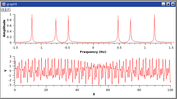
"FFT performed on a curve to extract the characteristic frequencies. The signal is on the bottom plot, while the amplitude-frequency plot is on the top layer."

"The signal is on the bottom plot, while the amplitude-frequency plot is on the top layer." [2]

Swiss Federal Institute of Technology Zurich

Swiss Federal Institute of Technology Zurich
Fast Fourier Transform
Numerical Analysis Seminar
Stefan W?orner

pdf: https://www.math.ethz.ch/education/bachelor/seminars/fs2008/nas/woerner.pdf

History

"The history of the Fast Fourier Transform (FFT) starts in 1805, when Carl Friedrich Gauss tried to determine the orbit of certain asteroids from sample locations. Thereby he developed the Discrete Fourier Transform (DFT), even before Fourier published his results in 1822. To calculate the DFT he invented an algorithm which is equivalent to the one of Cooley and Tukey. However, Gauss never published his approach or algorithm in his lifetime." [3]

Continuous Fourier Transform (CFT)
Discrete Fourier Transform (DFT)

Since the calculation of the DFT and the inverse DFT are almost equal, it follows, that a efficient method to calculate the DFT, as the FFT algorithm, can be used to calculate the inverse DFT, as well"

The recursive FFT algorithm is a classical divide and conquer algorithm

Recursive Implementation

Algorithm 1 - Recursive FFT

function y = fft_rec(x)
n = length(x);
if n == 1
  y = x;
else
  m = n/2;
  y_top = fft_rec(x(1:2:(n-1)));
  y_bottom = fft_rec(x(2:2:n));
  d = exp(-2 * pi * i / n) .^ (0:m-1);
  z = d .* y_bottom;
  y = [ y_top + z , y_top - z ];
end

Iterative Implementation

The iterative implementation of the FFT algorithm is not as straight forward as the recursive.

Algorithm 2 - Iterative FFT

function y = fft_it(x)
n = length(x);
x = x(bitrevorder(1:n));
q = round(log(n)/log(2));
for j = 1:q
  m = 2^(j-1);
  d = exp(-2 *pi * i /m).^(0:m-1);
  for k = 1:2^(q-j)
    s = (k-1)*2*m+1; % start-index
    e = k*2*m; % end-index
    r = s + (e-s+1)/2; % middle-index
    y_top = x(s:(r-1));
    y_bottom = x(r:e);
    z = d .* y_bottom;
    y = [y_top + z, y_top - z];
    x(s:e) = y;
  end
end

A gentle introduction to the FFT

A gentle introduction to the FFT - http://www.earlevel.com/main/2002/08/31/a-gentle-introduction-to-the-fft/

"The Fast Fourier Transform is an algorithm optimization of the DFT—Discrete Fourier Transform. The “discrete” part just means that it’s an adaptation of the Fourier Transform, a continuous process for the analog world, to make it suitable for the sampled digital world. Most of the discussion here addresses the Fourier Transform and it’s adaptation to the DFT. When it’s time for you to implement the transform in a program, you’ll use the FFT for efficiency. The results of the FFT are the same as with the DFT; the only difference is that the algorithm is optimized to remove redundant calculations. In general, the FFT can make these optimizations when the number of samples to be transformed is an exact power of two, for which it can eliminate many unnecessary operations."

"From Fourier we know that periodic waveforms can be modeled as the sum of harmonically-related sine waves. The Fourier Transform aims to decompose a cycle of an arbitrary waveform into its sine components; the Inverse Fourier Transform goes the other way—it converts a series of sine components into the resulting waveform. These are often referred to as the “forward” (time domain to frequency domain) and “inverse” (frequency domain to time domain) transforms. For most people, the forward transform is the baffling part—it’s easy enough to comprehend the idea of the inverse transform (just generate the sine waves and add them). So, we’ll discuss the forward transform; however, it’s interesting to note that the inverse transform is identical to the forward transform (except for scaling, depending on the implementation). You can essentially run the transform twice to convert from one form to the other and back!"

Fast Fourier Transform

Contents